|
|
Introduction to
LabVIEW
MathScript
by
12. May 2008
Contents:
1 Preface
2 Introduction
3
MathScript window (desktop math tool)
4 MathScript node (in a
LabVIEW Block diagram)
5 Learning the MathScript
language
6 MathScript
classes with functions and commands
6.1 Standard
MathScript classes
6.2 Control Design MathScript classes
6.3 Examples of using Control Design
functions
1 Preface
This document gives you an introduction to MathScript (for LabVIEW 8.5). It is assumed that you have basic LabVIEW skills.
This tutorial contains a number of activities that you are supposed to perform. These activities are shown in blue boxes, as here:
| Activities are shown in blue boxes as this one. |
Please send comments or suggestions regarding this document via e-mail to finn@techteach.no.
More LabVIEW stuff is available at Finn's LabVIEW Page.
2 Introduction
MathScript is a LabVIEW tool for executing textual mathematical commands (or expressions). Some features of MathScripts are:
- Matrix and vector based calculations (linear algebra)
- Visualization of data in plots
- Running scripts containing a number of commands written in a file
- A large number of mathematical functions. An overview is given later in this document.
- MathScript command are equal to MATLAB commands (but some MATLAB commands may not be implemented).
MathScript can be used in two ways (both are described in the following sections):
- In a MathScript window which actually can be used as a desktop mathematical tool independent of LabVIEW, although it is opened via the menu in LabVIEW.
- In a MathScript node which appears as a frame inside the Block diagram of a VI, as the Formula node. A MathScript node is available on the palette.
MathScript can not be run on a real-time target, as FieldPoint RT.
3 MathScript window (desktop math tool)
A MathScript window is opened via the menu in LabVIEW, see the figure below.
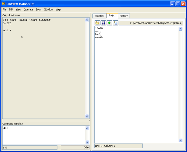
The MathScript window
The MathScript window consists of a number of (sub)windows:
- The Command Window where you type the commands to be executed (after you press the Enter key)
- The Output Window where executed commands and numerical results are shown.
- The Workspace window, which contains the Variables, Script,
and History (sub)windows
containing the following tabs:
- Variables: Lists generated variables. The numerical value of these variables can be displayed. The value can also be plotted graphically by selecting Graphics First in the Variables dialog window.
- Script: Opens a script editor. To open another Script editor: Select the menu (in the MathScript window) .
- History: Shows a list of previous commands that you have executed.
The Workspace window contains a number of buttons:
- Open (script)
- Run runs the present code in the editor, even if the script has not been saved. Running includes compiling the code (i.e. generating executable code), before it is run (executed). Note that the script is not saved with the Run button.
- Save (script)
- New (script)
The Workspace window can be closed via the menu in the MathScript window.
|
4 MathScript node (in a LabVIEW Block diagram)
You can include MathScript commands in the Block diagram of a VI in a MathScript node which is available on the palette. Let us look at a simple example. Below are the Front panel and the Block diagram of mathscript_example.vi, followed by comments. You will soon be guided through the development of this VI.
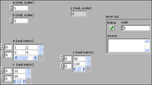
Front panel of mathscript_example.vi
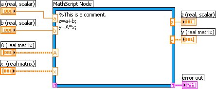
Block diagram of mathscript_example.vi
Comments to the Front panel:
-
To the left of the Front panel are the scalar controls (or numbers in DBL (double) formal), a and b, and two real matrices, A and x.
-
Further to the right are indicators, z and y. z is a real scalar. y is a real matrix.
-
error out is a cluster indicator displaying any MathScript errors on the Front panel.
Comments to the Block diagram:
-
a, b, A, and x are names of the inputs to the MathScript. The data type of a and b are real scalars (we may also say doubles). A and x are real matrices.
-
Matrices are used, not arrays, in these matrix based calculations! Connecting arrays to the MathScript node in stead of matrices in such applications will cause an error.
Scalars and matrices are probably the most common data types in MathScript applications. However, you can also use arrays and strings (text). The data type of a MathScript node input or output are set via right-clicking on the input/output, and selecting the sata type from a list.
-
The MathScript contains an error cluster output which here is wired to a front panel indicator. It is wise to include an error cluster in the early stage of the development of a VI containing a MathScript node as it helps you to find errors. These error may otherwise be quite hard to find.
The MathScript node contains three commands: One comment, which starts with a percent sign, and two ordinary commmands separated by semicolon.
Note: If you want to include a matrix constant in the Block diagram, you may face trouble because there is no matrix constant on the Functions palette (this is a little strange...). In this case, you may in stead intermediately create a matrix control on the Front panel, and then change its Block diagram terminal from control to constant via right-click on the terminal. If you really want to use matrix constants in the Block diagram, you may consider creating or defining the matrix directly in the MathScript node. For example you can type
M = [1,2;3,4]
which creates a 2x2 matrix with 1 and 2 in the first row, and 3 and 4 in the second row.
Now, it's your turn. To create a VI similar to mathscript_example.vi:
Save the VI, and run it. Does it work? Note: This VI will run the code once since the code is not inside any While loop. If you want, you can add a While loop, a Stop button, and a Metronome. If you do not want to add a While loop, but still want to run your VI continuously while testing it, click the Run Continuously button in stead of the Run button in the toolbar. |
5 Learning the MathScript language
Below is a number of commands that will teach you the basics of the MathScript language.
StartupOpen the MathScript window (menu ). To get more space in the MathScript window, close the Workspace window (via the View menu in the MathScript window). Execute the following commands in the Command window (by pressing the Enter button on the keyboard), and observe the results in the Output window. Below the commands are written in bold. Entering commandsHere is a simple calculation:
The result is 3 (as you might have guessed) which is assigned to the standard variable ans (short for answer). ans always holds the result of the last command. To add 4 to ans:
ans now gets value 7. Several commands may be written on one line, separating the commands using either semicolon or comma. With semicolon the result of the command is not displayed in the Output window, but the command is executed. With comma the result is displayed.
With the above commands the value of a is not displayed, while the values of b and c are displayed. Recalling previous commandsTo recall previous commands, press the Arrow Up button on the keyboard as many times as needed.
To recall a previous command starting with certain characters, type these characters followed by pressing the Arrow Down button on the keyboard. Try recalling the previous command(s) beginning with the a character:
Case sensitivityMathScript is case sensitive:
MathScript says that C (capital) is an unknown symbol although the c (lowercase) variable exists. Formating the outputSometimes the output of a command is a large amount of numbers and/or text. It may be convenient, then, to show the results wrapped in the Output window. As a start, make the following menu selection in the MathScript window: (so that the output is wrapped). Now, type the following command:
Certainly the output is wrapped. Now, make the menu selection so that the output is not wrapped (the same menu as above), and then repeat the command:
The output is not wrapped. I suggest you now select wrapping the output. HelpAbove you used the help command. It command displays information about a known command, typically including an example. Try
You can also search for information about a command via the menu in the MathScript window:
Number formatsThe format command is used to select between different formats of the output, cf. the information about the format command that you saw above. Try the following commands:
In most cases format short is ok. This is also the default format. To reset to format short:
Entering numbersYou can enter numbers in various ways:
The WorkspaceAll variables generated in a MathScript session (a session lasts between launching and quitting MathScript) are saved in the MathScript Workspace. You can see the contents of the Workspace using the menu . Alternatively, you can use the who command:
You can delete a variable from the Workspace:
The Workspace is cleared if you quit MathScript. You can however save variables in the Workspace into a file using the Save command, and restore the variables using the load command. (If you generate the variables by running commands in a MathScript script, it may be sufficient to just save the script, not the variables, and run the script when you need the variables.) The MathScript Working Directory is the default folder when using the save or load commands. You can display, and change, the Working Directory via the menu, but you do not have to do this unless you are going to use the save or load commands. As an alternative to displaying the Working Directory using the menu, you can also display the Working Directoy using the pwd command (Print Working Directory):
And you can change the Working Directory using the cd command. MathScript functions are polymorphic, i.e. they typically take both scalars and vectors (arrays) as arguments. As an example, the following two commands calculate the square root of the scalar 2 and the square root of each of the elements of the vector of integers from 0 to 5, respectively:
When the argument is a vector as in this case, the calculation is said to be vectorized. Matrices and vectorsThe matrix is the basic data element in MathScript. A matrix having only one row or one line are frequently denoted vector. Below are examples of creating and manipulating matrices (and vectors). To create a matrix, use comma to separate the elements of a row and semicolon to separate columns. For example, to create a matrix having numbers 1 and 2 in the first row and 3 and 4 in the second row:
with the result A = To transpose a matrix use the apostrophe:
To create a row vector from say 0 to 4 with increment 1:
To create a row vector from say 0 to 4 with increment 0.5:
To create a column vector from say 0 to 4 with increment 1:
You can create matrices by combining vectors (or matrices):
Here are some special matrices:
You can address an element in a matrix using the standard (row number, column number) indexing. Note: The element indexes starts with one, not zero. (In LabVIEW, array indexes starts with zero....) For example (assuming matrix A=[1,2;3,4] is still in the Workspace), to address the (2,1) element of A and assign the value of that element to the variable w:
with result w=3. You can address one whole row or column using the : (colon)operator. For example,
with result C2=[3,4] (displayed a little different in the Output window, though). Element-by-element calculationsElement-by-element calculations are executed using the dot operator together with the mathematical operator. Here is an example of calculating the product of each of the elements in two vectors:
with result [4 10 18]. ScriptsCreate a script in the Script editor (which is on the Script tab in the Workspace window (a new Script editor can opened via the menu ) of name script1.m with the following contents:
Save the script in any folder you want. Run the script by clicking the Run button. All the commands in the script are executed from top to bottom as if they were entered at the command line. You should make it a habit to use scripts for all your work. In this way you save your work, and you can automate your tasks. PlottingYou can plot data using the plot command (several addition plotting commands are available, too). Here is an example: Generate a vector t of assumed time values from 0 to 100 with increment 0.1:
Generate a vector x as a function of t:
Generate a vector y as a function of t:
Open Figure no 1:
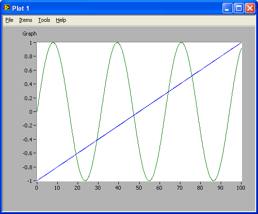
Plots x verus t, and y versus t, in the same graph:
The resulting plot is shown in the figure below.
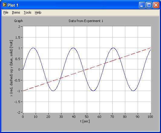
The resulting plot Probably you want to add labels, annotations, change line color etc. This can be done using menus in the Plot window. This is straightforward, so the options are not described here. As an alternative to setting labels etc. via menus in the Plot window, these can be set using commands. Below is an example, which should be self-explaining, however note how the attributes to each curve in the plot is given, see the plot() line in the code below. t=[0:.1:100]';
Plot generated by command-based configuration of the plot
|
6 MathScript classes with functions and commands
The MathScript functions and commands are grouped into classes. The standard classes are classes inherent in "basic" MathScript. If some LabVIEW toolkits are installed, e.g. Control Design Toolkit, additional MathScript classes are installed. Classes can be listed using LabVIEW Help.
6.1 Standard MathScript classes
The table below shows standard MathScript classes.
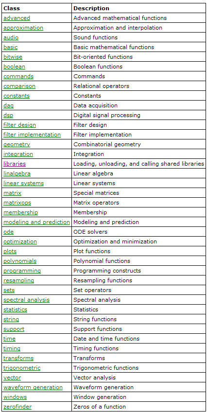
MathScript classes of functions and commands
Opening a class by clicking the its hypertext, shows the individual functions or commands in that class. The figure below shows as an example the functions in the trigonometric class.
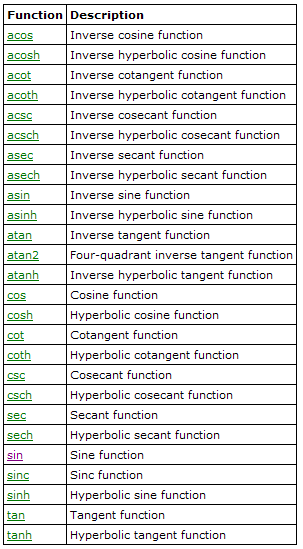
The functions in the trigonometric class
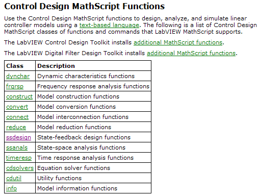
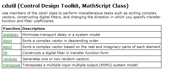
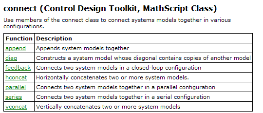
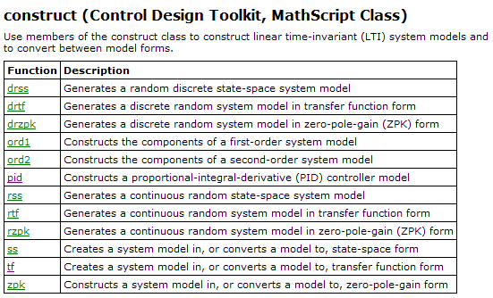
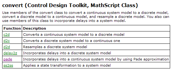
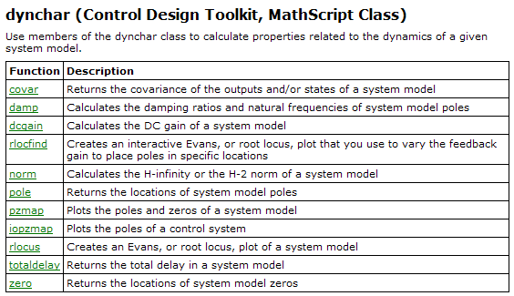
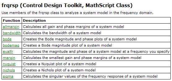
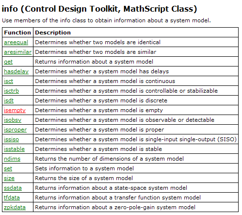
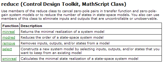
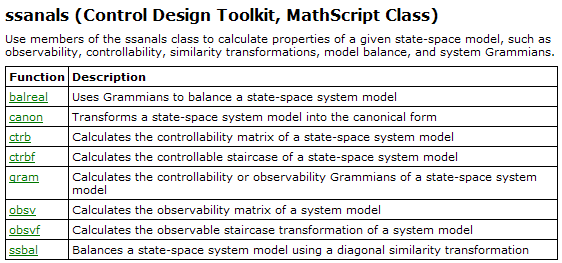
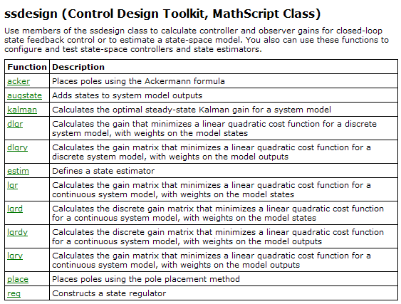
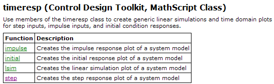
6.2 Control Design MathScript classes
By installing Control Design Toolkit additional MathScript classes are installed, see below.
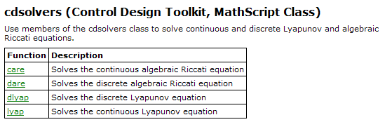
In the following are shown (in alphabetic order) the individual functions of the Control Design classes shown above.
6.3 Examples of using Control Design functions
In the follwing are some basic examples of using Control Design functions.
6.3.1 Defining and simulating a s-transfer function
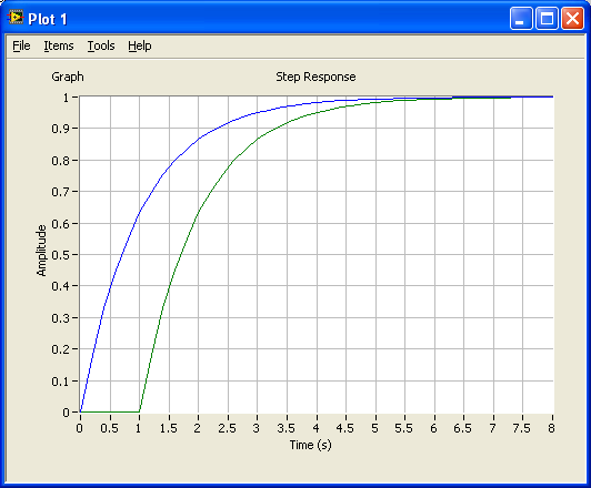
Enter and then run the following script in the Script editor. The script defines two s-transfer functions using the tf function, and simulates their step responses using the step function.
|
s=tf('s'); %Defines s to be the Laplace variable used in transfer functions K=1; T=1; %Gain and time-constant H1=tf(K/(T*s+1)); %Creates H as a transfer function delay=1; %Time-delay H2=set(H1,'inputdelay',delay);%Defines H2 as H1 but with time-delay figure(1) %Plot of simulated responses will shown in Figure 1 step(H1,H2) %Simulates with unit step as input, and plots responses. |
The figure below shows the responses.
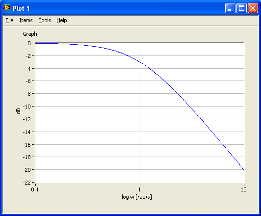
6.3.2 Calculating and plotting frequency response in a Bode plot
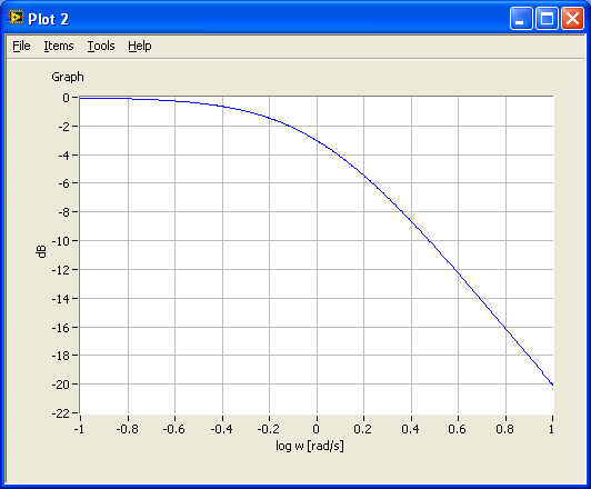
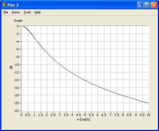
The bode function plots frequency response in a Bode plot. In the script below three various, alternative, ways to display the magnitude (amplitude gain) data are shown. Most information is displayed with the third alternative, the plot command (at the bottom of the script).
|
s=tf('s'); %Defines s to be the Laplace variable used in transfer functions K=1; T=1; %Gain and time-constant H1=tf(K/(T*s+1)); %Creates H1 as a transfer function w_min=0.1; %Min freq in rad/s w_max=10; %Max freq in rad/s [mag,phase,w_out]=bode(H1,[w_min,w_max]); %Calculates frequency response figure(1) semilogx(w_out, 20*log10(mag)), grid, xlabel('log w [rad/s]'),ylabel('dB')%Plots frequency response figure(2) plot(log10(w_out), 20*log10(mag)), grid, xlabel('log w [rad/s]'),ylabel('dB')%Plots frequency response figure(3) plot(w_out, 20*log10(mag)), grid, xlabel('w [rad/s]'),ylabel('dB')%Plots frequency response |
The figures below show the plots.
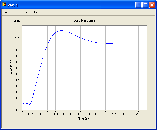
6.3.3 Frequency response analysis and simulation of feedback (control) systems
The script below shows how you can analyze a control system. In this example, the process to be controller is a time-constant system in series with a time-delay. The sensor model is just a gain. The controller is a PI controller.
The time-delay is approximated with a rational transfer function (on the normal numerator-denominator form). This is necessary when you want to calculate the tracking transfer function and the sensitivity transfer function automatically using the feedback function. The time-delay approximation is implemented with the pade function (Padé approximation).
- First, the models are defined using the tf function. The time-delay is approximated using the pade function.
- The control system is simulated using the step function.
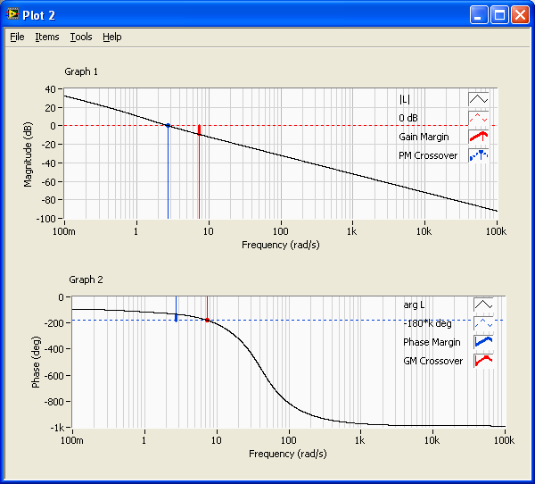
- The stability margins and corresponding crossover frequencies are calculated using the margin function.
- The control system transfer functions - namely the loop transfer function, tracking transfer funtion and the sensitivity transfer function - are calculated using the series function and the feedback function.
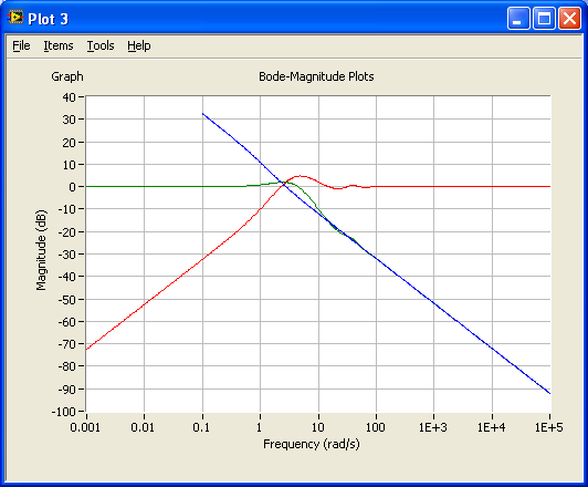
- These transfer functions are plotted in a Bode diagram using the bode function.
Although the system in this example is a continuous-time system, discrete-time systems can be analysed in the same way. (With a discrete-time system, no Padé-approximation is necessary because time-delays can be precisely represented in the model.)
|
s=tf('s'); %Defines s to be the Laplace variable used in transfer functions %Defining the process transfer function: K=1;T=1;Tdelay=0.2; %Process parameters padeorder=5; %Order of Pade-approximation of time-delay. Order 5 is usually ok. P1=set(tf(K/(T*s+1)),'inputdelay',Tdelay);%Including time-delay in process transfer function P=pade(P1,padeorder);%Deriving process transfer function with Pade-approx of time-delay %Defining sensor transfer function: Km=1; S=tf(Km); %Defining sensor transfer function (just a gain in this example) %Defining controller transfer function: Kp=2.5; Ti=0.6; C=Kp+Kp/(Ti*s); %PI controller transfer function %Calculating control system transfer functions: L=series(C,series(P,S)); %Calculating loop tranfer function M=feedback(L,1); %Calculating tracking transfer function N=1-M; %Calculating sensitivity transfer function %Analysis: figure(1) step(M), grid %Simulating step response for control system (tracking transfer function) %Calcutating stability margins and crossover frequencies: [gain_margin, phase_margin, gm_freq, pm_freq] = margin(L) %Note: Help margin in LabVIEW shows erroneously parameters in other order than above. figure(2) margin(L), grid %Plotting L and stability margins and crossover frequencies in Bode diagram figure(3) bodemag(L,M,N), grid %Plots maginitude of L, M, and N in Bode diagram |
The figures below show the three plots generated by the above script.