|
|
|
Introduction
to
Simulation Module for LabVIEW 8.5
by
1. March 2008
Contents:
1 Preface
2 Introduction
3 The contents of the
Simulation functions palette
4 An example:
Simulator of a liquid tank
4.1
Developing the mathematical model of the system to be simulated
4.2 The
Front panel and the Block diagram of the simulator
4.3
Configuring
the simulation
5 Various topics
5.1
Representing state space models using Formula node and integrators
5.2 Creating subsystems
5.3 Getting a linearized model of a subsystem
5.4
Simulating control systems
5.5 Converting models between Simulation Module and Control Design Toolkit
5.6
Putting code into a While loop running in parallell with a Simulation loop
5.7 Translating SIMULINK models into LabVIEW Simulation models
1 Preface
This document gives an introduction to the LabVIEW Simulation Module for LabVIEW 8.5. It is assumed that you have basic skills in LabVIEW programming. There are tutorials for LabVIEW programming available from the National Instruments' webside http://ni.com, and I have made one myself (to serve the needs in my own teaching more specifically), see Finn's LabVIEW Page.
This tutorial contains a number of activities that you are supposed to perform. These activities are shown in blue boxes, as here:
| Activities are shown in blue boxes as this one. |
Please send comments or suggestions to improve this tutorial via e-mail to finn@techteach.no.
More tutorials that may be relevant for you as a LabVIEW user are available from Finn's LabVIEW Page.
2 Introduction
The LabVIEW Simulation Module is a block diagram based environment for simulation of linear and nonlinear continuous-time and discrete-time dynamic systems. Many simulation algorithms (i.e. numerical methods for solving the underlying differential equations) are available, e.g. various Runge-Kutta methods. The mathematical model to be simulated must be represented in a simulation loop, which in many ways is similar to the ordinary while loop in LabVIEW. You can make the simulation run as fast as the computer allows, or you can make it run with a real or scaled time axis, thus simulating real-time behaviour, with the possibility of the user to interact with the simulated process. The simulation loop can run in parallel with while loops within the same VI.
3 The contents of the Simulation functions palette
Once the Simulation Module is installed, the Simulation palette is available from the Functions palette. The Simulation palette is shown in the figure below.
|
Open the Block diagram of a blank VI. Open the Simulation palette as follows: . The figure below shows this palette. Browse the palettes on the Simulation palette. Read the information about each of the palettes provided below. Close the VI without saving it. |
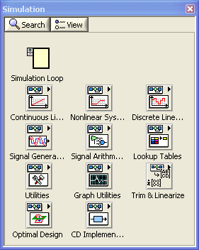
The Simulation Palette on the Functions Palette
Below is an overview over the functions and possible subpalettes on the Simulation Palette.
- Simulation Loop, which defines the borders of the simulation diagram on which the simulation functions are placed. Note that (most of) the functions found on the Simulation palette can be placed only inside a simulation loop.
- Continuous palette containing the following functions and/or
subpalettes:
- Zero-Pole-Gain Function Space Delay
- Derivative
- Time Delay
- State Space
- Transfer Function
- Zero-Pole-Gain
- Nonlinear palette containing the following functions:
- Backlash
- Friction
- Quantizer
- Dead Zone
- Rate Limiter
- Relay
- Saturation
- Switch
- Zero Cross Detection
- Discrete palette containing the following functions:
- Discrete Integrator
- Discrete Unit Delay
- Discrete Zero-Order Hold
- Discrete First-Order-Hold
- Discrete State Space
- Discrete Transfer Function
- Discrete Zero-Pole-Gain
- Discrete Filter
- Signal Generation palette containing the following functions:
- Chirp Signal
- Ramp
- Pulse
- Signal Generator
- Sine Wave
- Step
- Indexer, which is used to index an array or waveform (like the ordinary array indexing function in LabVIEW) by the current simulation time.
- Signal Arithmetic palette containing the following functions:
- Gain
- Summation, with any number of inputs. Inputs may also be subtracted.
- Multiplication, with any number of inputs. Inputs can slo be used as divisors.
- Lookup Tables palette containing the following functions, which may be
used to look up values from arrays of tabular (e.g. experimental) data:
- Lookup Table 1D (dimension one)
- Lookup Table 2D (dimension two)
- Lookup Table 3D (dimension three)
- Utilities palette containing the following functions:
- Collector, which collects a signal at each time step of the simulation and outputs a history of the signal value and the time at which this function recorded each value in the history. The Collector builds an array on its output from the input it recieves at each simulation step.
- Memory, which stores the value of the Input signal from the previous iteration of the simulation. You can use this function to transfer values from one iteration of the Simulation Loop to the next.
- Indexer, which is used to index an array or waveform (like the ordinary array indexing function in LabVIEW) by the current simulation time.
- Simulation Parameters, which can be used to read or get (not set) simulation parameters.
- Simulation Time, whose output is the simulation time. It works like a simulation clock.
- Report Sim Error
- Halt Simulation, which stops the simulation when its input becomes False.
- Graph Utilities palette containing the following functions:
- SimTime Waveform, which is used to plot simulated variables continuously in a LabVIEW Chart. When this function is put into the simulation loop, a Chart is automatically attached to the function.
- Buffer XY Graph, which is used to collect arrays of signals to be plotted in a LabVIEW Graph. When this function is put into the simulation loop, a Graph is automatically attached to the function.
- Trim & Linearize palette containing several functions for calculating an operating point and to have LabVIEW develop a linear model in that operating point.
- Optimal Design palette containing functions to calculate optimal PID settings for a process model from an objective function (optimization criterion).
- CD Implementation palette containing functions to calculate state estimations using a Kalman Filter. (CD = Control Design. The same functions are found on the CD palette, too.)
4 An example: Simulator of a liquid tank
In this section we will study and partly develop a simulator of a liquid tank. Actually, we will play with a premade example, but not develop it from scratch. I think this is an effective way to learn using the Simulation module, assuming that you have basic skills in LabVIEW programming. You are supposed to have basic knowledge about modeling of dynamic systems, as described in e.g. Dynamic Systems - modelling, analysis and simulation or in any other book about dynamic systems theory.
4.1 Developing the mathematical model of the system to be simulated
The system to be simulated is a liquid tank, see the figure below. The simulator will calculate and display the level h at any instant of time. The simulation will run in real time, with the possibility of scaled real time, thereby giving the feeling of a "real" system. The user can adjust the inlet by adjusting the pump control signal, u.
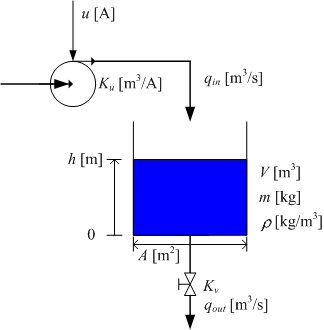
Liquid tank
Any simulator is based on a mathematical model of the system to be simulated. Thus, we start by developing a mathematical model of the tank.
We assume the following (the parameters used in the expressions below are defined in the figure above):
- The liquid density is the same in the inlet, in the outlet, and in the tank.
- The tank has straight, vertical walls.
- The liquid mass and level are related through
m(t) = ρAh(t)
- The inlet volumetric flow through the pump is proportional to the pump
control signal:
qin(t) = Kuu(t)
- The outlet volumetric flow through the valve is proportional to the square
root of the pressure drop over the valve. This pressure drop is assumed to be
equal to the hydrostatic pressure at the bottom of the tank (sqrt means square
root):
qout(t) = Kvsqrt[ρgh(t)]
Mass balance (i.e., rate of change of the mass is equal to the inflow minus the outflow) yields the following differential equation:
dm(t)/dt = ρqin(t) - ρqout(t)] (1)
or, using the above relations,
d[ρAh(t)]/dt = ρKuu(t) - ρKvsqrt[ρgh(t)] (2)
We will now draw a mathematical block diagram of the model. This block diagram will then be implemented in the block diagram of the simulator VI. As a proper starting point of drawing the mathematical block diagram, we write the differential equation as a state-space model, that is, as a differential equation having the first order time derivative alone on the left side. This can be done by pulling ρ and A outside the differentiation, then dividing both sides by ρA. The resulting differential equation becomes
d[h(t)]/dt = (1/A)*{Kuu(t) - Kvsqrt[ρgh(t)]} (3)
This is a differential equation for h(t). It tells how the time derivative dh(t)/dt can be calculated. h(t) is calculated (by the simulator) by integrating dh(t)/dt with respect to time, from time 0 to time t, with initial value h(0), which we here denote hinit. To draw a block diagram of the model (3), we may start by adding an integrator to the empty block diagram. The input to this integrator is dh/dt, and the output is h(t). Then we add mathematical function blocks to construct the expression for dh/dt, which is the right side of the differential equation (3). The resulting block diagram for the model (3) can be as shown in the figure below.
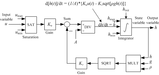
Mathematical block diagram of Differential Equation (3)
The numerical values of the parameters are shown in the front panel picture below.
We will assume that there are level alarm limits to be displayed in the simulator. The limits are
AH_h = 0.9m (Alarm High)
AL_h = 0.1m (Alarm Low)
The block diagram developed above will be implemented in a Simulation Loop in the Block diagram of our simulation VI.
4.2 The Front panel and the Block diagram of the simulator
The subsequent figures show the front panel and the block diagram of the complete VI, tanksim.vi.
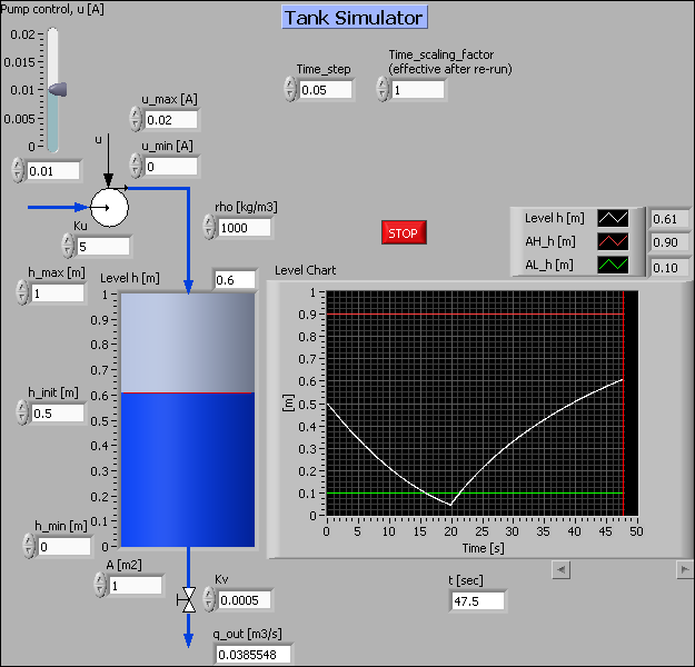
Front panel of tanksim.vi.
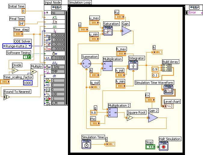
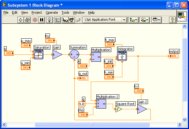
Block diagram of tanksim.vi.
|
Open
tanksim.vi, and save it with the name
my_tanksim.vi in any folder you prefer. Run the VI, and play with controls on the Front panel as you wish. Try adjusting the Time_scaling_factor (the VI must be stopped and started again to make any change of this element become effective). Finally, stop the VI. Read the comments to the Front panel given below. |
In the following, you are asked to remove, and then re-insert elements to the Front panel and the Block diagram of my_tanksim.vi. The purpose of this is to learn how to develop a simulator of a simulator of realistic complexity in Simulation Module, without starting completely from scratch. I guess this is an effective way of learning. It assumes that you have basic LabVIEW programming skills, as pointed out in the Preface.
The Front panel
- The Tank indicator is copied from the Numeric palette (on the Controls
palette).
It is assumed that my_tanksim.vi is open. Note the Label and the Caption of the Tank indicator. Remove the Tank indicator from the Front panel. Then insert a new one at the same place, with same Label and Caption. Open the Block diagram. Connect the Tank indicator terminal to the Integrator output, which represents the level.
Check that the VI is without errors. Then save it. Run it, and finally stop it.
- The numeric controls, e.g. the vertical pointer slide, are copied from the Numeric palette.
- The pump and the valve pictures are graphical object which I have
originally created in the Visio tool for technical drawings. Here are
EMF-files (Enhanced Meta Files) of these objects:
pump.emf and
valve.emf.
Open the Front panel of my_tanksim.vi. Remove the pump picture. Download pump.emf to any folder. Insert the pump picture as follows: Select the following menu in LabVIEW: , and select the downloaded pump.emf file. Then, paste the file into the Front panel at a proper place with . Resize the picture properly.
If a picture overlaps one or more control elements on the front panel, it may not be possible to adjust these controls. To avoid this situation it is necessary to put the picture to the background layer of the Front panel. This is done via the Reorder button in the toolbar.
Select the pump picture (by clicking it). Then Click the Reorder button in the toolbar / Select Move to Back. Save the VI.
- The pipelines are copied from the Decorations palette. The color is set to
blue using the Set Color button on the Tools palette, which is opened via the
menu.
Remove the pipeline entering the Tank indicator. Then add a new pipeline, and give it a blue color. Save the VI.
- The chart is not copied directly onto the front panel from the Graph palette. In stead it is created on the front panel via the block diagram, see the comments to the Block diagram below.
The Block diagram
| Open the Block diagram of my_tanksim.vi. Try to identify the corresponding elements in the mathematical block diagram and the Block diagram of my_tanksim.vi (select one block at a time in the mathematical block diagram and find the corresponding element in the VI Block diagram). |
Here are comments and activities for various part of the Block diagram:
- The Simulation loop contains the blocks
or functions representing the mathematical
model of the tank. A Simulation loop looks like a While loop, but is not
the same. The Simulation loop runs a simulation according to the simulation
configurations. A While loop just executes the code placed inside the loop.
Add a Simulation loop at an empty place outside the existing Simulation loop. The Simulation loop is on the Simulation palette. (Do not remove the existing loop since many elements are wired to its Input Node to the left.) Then remove this new Simulation loop. - The Integrator function performs time-integration of the input to
the function.
Open the Configuration window of the Integrator block by double-clicking the block. The figure below shows the Integrator Configuration window. 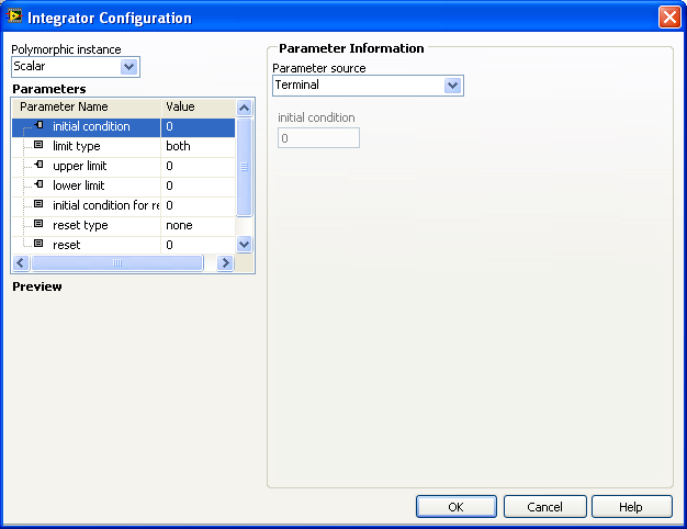
Configuration window of the Integrator block. The window is opened by double-clicking the block.
Here are comments to the Integrator Configuration window: The Parameters field contains a number of parameters that can be configured. Once you have selected a parameter in the list, you have two options in the Parameter source field:
- By selecting Configuration Dialog Box, which is the default option, you can set the value of the selected parameter directly in the dialog box. This is an internal setting of the parameter.
- By selecting Terminal an input terminal is created on the left part of the block in the Simulation Loop, and you can wire a value of the correct data type to that input. This is an external setting of the parameter. In our VI the following parameters have been set externally: Initial condition; Upper Limit; Lower Limit. The terminals wired to these three block inputs are h_max, h_min, and h_init, as you can see from the block diagram picture.
Remove the existing Integrator function in the Block diagram. Then, insert a new Integrator function from the Continuous palette at the same place, with the same configuration as for the original Integrator function, cf. the description above. Ensure the VI is without errors, then save the VI.
-
The Summation function can be configured to perform both summation and subtraction.
Open the Configuration window of the Summation block by double-clicking the block. The figure below shows the Summation Configuration window. Ensure the VI is without errors, then save the VI.
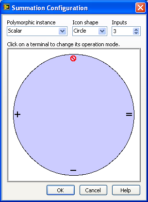
Configuration window of the Summation block
Here are comments to the Summation Configuration window: You can select the number of inputs via the Inputs list, and select Add or Subtract or Disable for each input (by clicking on the symbols inside the circle). You can also select among Rectangle and Circle Icon shape, and wether the input is a scalar (single signal) or a vector (multiple signals).
Remove the existing Summation function in the Block diagram. Then, insert a new Summation function from the Signal Arithmetic palette at the same place, with the same configuration as for the original Summation function, cf. the description above. Ensure the VI is without errors, then save the VI.
-
The Multiplication function is configured in a similar matter as the Summation block. You can add and remove inputs, and select Multiply or Divide or Disable for each input.
Open the Configuration window of the Multiplication block by double-clicking the block. Note the settings. Remove the existing Multiplication function in the Block diagram. Then, insert a new Multiplication function from the Signal Arithmetic palette at the same place, with the same configuration as for the original Multiplication function.
Ensure the VI is without errors, then save the VI.
-
The Square Root function is copied from the standard Numeric palette. So this is an example of including a block or function which is contained in a palette outside the Simulation palette. In general, functions from other palettes can be used inside a Simulation Module.
Remove the Square Root function from the Block diagram. Then add a Square Root function at the same place, and wire its input and output. Ensure the VI is without errors, then save the VI.
-
The Build Array function is copied from the ordinary Array palette. It is used to collect the three signals to be plotted in the Chart to be described below), namely the level (being the output from the Integrator, and the two constants 0.9 and 0.1). Now, may be you think: Why using a Build Array function? In a While loop we use a Bundle function to collect the signals. To this question National Instrument answers that the implementation of the Simulation Loop requires a Build Array function to be used.
-
Although it is not used in our VI, you may flip a block by right-clicking the block and selecting Reverse terminals in the menu that is opened.
Remove the existing Build Array function in the Block diagram. Then, insert a new Build Array function at the same place, expand the number of inputs to three (by dragging the bottom line of the block downwards or by right-clicking the block and selecting Add Input in the menu that is opened). Ensure the VI is without errors, then save the VI.
-
The SimTime Waveform function is copied from the Graph Utilities palette. When you insert a SimTime Waveform block into a simulation diagram, a Waveform Chart is automatically created on the front panel. Due to this block the time axis on the Waveform Chart automatically shows the simulation time, so you do not have to define the Multiplier paramter in the Scale tab in the Property window of the Chart (as you would have to with a Chart in an ordinary While loop). However, the default time format is Absolute Time which is not particularly convenient since it displays 1.1.1904 as a reference time. I suggest using the Floating point format in stead (this is set in the Format & Precision tab of the Property window of the Waveform Chart).
The Chart is automatically emptied before the VI starts running, so you do not have to create any Property node for this Chart for this purpose (using Property nodes to configure Charts is described here).
Remove the existing SimTime Waveform function and the Chart terminal in the Block diagram. Then, insert a new SimTime Waveform function together with a Chart Build at the same place, and connect the SimTime Waveform to the Build Array function output. Configure the Chart properly via its Property window (opened via right-clicking the Chart on the Front panel). Ensure the VI is without errors, then save the VI.
At the left part of the block diagram, outside the Simulation Loop, is code used to configure the simulation. How to configure the simulation is explained in the following section.
4.3 Configuring the simulation
Simulation configuration is about selecting parameters as initial simulation time, final simulation time, numerical method, time step etc. The configuration can be done in two ways:
- Programmatically: By wiring values to the Input Node of the Simulation Loop, see the left part of the block diagram.
- By a dialog window: In the Configure Simulation Parameters dialog window which is opened by right-clicking the simulation loop border and selecting the menu Configure Simulation Parameters
The setting defined programmatically overrides the settings made in the dialog window. Since the programmatic method gives more flexibility and the settings are clearly shown in the block diagram itself, I prefer the programmatic method.
Both configuration methods are described in the following sections.
Programmatic setting of simulation parameters
By expanding the Input Node outside the left part of the Simulation Node (by pulling the bottom of the node downwards), all parameters become available. The parameters are shown in the block diagram picture. To display the details somewhat better an expanded extract of that block diagram is shown in the figure below.
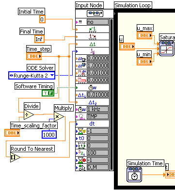
The Input Node of the Simulation Loop
Here are comments to the parameters that are wired:
- The Intial Time defines the initial simulation time, typically zero.
- The Final Time defines the simulation time when the simulation will stop. In our VI the final time is set to Inf (infinity). Will the simulation never stop, then? It will stop, due to the Halt Simulation function in the block diagram. When the user clicks the Stop button on the front panel the Halt Simulation function will cause the simulator to stop.
-
The Time Step is the resolution of the simulation time scale, see the figure below.
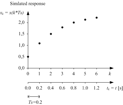
The time step is the resolution of the simulation time scale
In general, the smaller time step the better accuracy, but the larger the total number of calculations needed to calulate the simulated response for a given simulation time range. The main rule of selecting the time step is: Select the largest time step that does not influence the accuracy of the simulated response. You may iterate to find this largest time step. Start with some initial guess of the time step, and try increased values until you observe that the response is influenced by the time step. As an initial guess you may select the time step as
Ts = 0.1*Tmin
where Tmin is the smallest time constant of the model. If I do not know the smallest time constant, I set h = 0.05s which gived a fairly smooth update of the plotted simulation response on the screen.
- The ODE Solver is the numerical method used
to calculate - or solve for - the values of the state variables of the model.
(ODE is abbreviation for Ordinary Differential Equation.) In general, the
simpler solver, the less burden on the LabVIEW and the computer to perform the
simulation, but also, unfortunately, the less accuracy of the simulated response. This
selecting the solver method is a trade-off. It is my experience that using the
Runge-Kutta second order method (with a fixed time step) works fine in
most situations. (This method is quite similar to numerical integration using
the trapezoid rule.)
There are fixed-step solvers and variable-step solvers. In variable-step solvers LabVIEW automatically calculates the time step. However, it is my experience that the simulation runs smoother and that is it easier to post-process the simulation data if you use a fixed-step solver. Therefore I suggest using a fixed-step solver.
- Software Timing set to True makes LabVIEW run the simulation as fast as it can, i.e. the simulation time is not equal to the real time. Software Timing set to False gives you the possibility to set how fast the simulation will run. This is done with the Period parameter described below.
- The Discrete Time Step is the time step used for simulating dicrete-time functions (blocks). In the block diagram of our example the discrete time step is the Δtz parameter. Examples of discrete-time functions are discrete-time signal filters. Typically the discrete time step is set equal to the simulation time step, as in our example.
- The Period is the amount of real time between
two subsequent simulated time points. By setting the Period equal to the
simulation time step, Ts, the simulation runs in real time. By giving the Period
some other value, the simulation time scale is proportional to real
time. For example, if the simulation time step is 0.05s, setting Period equal to
0.01s causes the simulation to run 5 times faster than real time (thereby
speeding up the simulation for a slow system), while setting Period equal to
0.25s causes the simulation to run 5 times slower than real time (thereby
slowing down the simulation for a fast system).
Setting Period to 0 causes LabVIEW to run the simulation as fast as possible (on the given computer).
Note that on a PC Period is the number of milliseconds, since the PC clock runs with a frequency of 1kHz. For example, Period = 10 corresponds to Period equal to 0.01s. (It is however possible to use some other (faster) timing source than the PC clock.)
In our example the Period is calculated from the Time Step by dividing the Time Step by the terminal labeled Time_scaling_factor. The user can adjust the value of Time_scaling_factor on the front panel. The Round to Nearest (integer) function is used to make the result of the division an integer.
|
Disconnect each of the wires now connected to the Input Node of the
Simulation loop, and remove brolen wires (keyboard shortcut Ctrl + B). Then,
reconnect each of them, cf. this figure. Ensure the VI is without errors, then save the VI. |
Setting simulation parameters in a dialog window
By right-clicking on the border of the Simulation loop and selecting Configure Simulation Parameters in the menu that is opened, the Configure Simulation Parameters dialog window with the Simulation Parameters tab is opened, see the figure below.
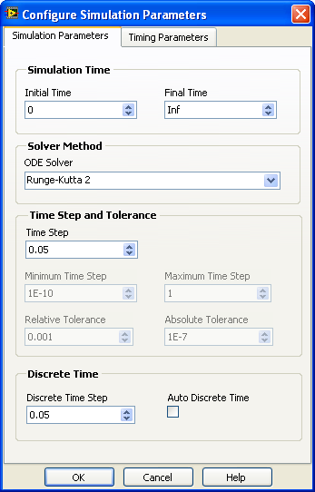
The Simulation Parameters tab in the Configure Simulation Parameters dialog window
| Open the Configure Simulation Parameters dialog window, and locate the parameters described below, but do not make any changes to the existing settings. Then, click the Cancel button. |
Most of the setting parameters in the Simulation Parameters tab are as for the programmatic parameter settings describe above, and the descriptions are not repeated here. Here are some additional comments:
If Auto Discrete Time is selected, the Discrete Time Step is automatically set equal to the simulation time step if you use a fixed-step solver, but it is automatically set to the initial time step for variable-step solvers. By default Auto Discrete Time is selected. I suggest that you uncheck the Auto Discrete Time checkbox and set the Discrete Time Step explicitly. (This corresponds to the wiring in the programmatic configuration.)
The figure below shows the Timing Parameters tab.
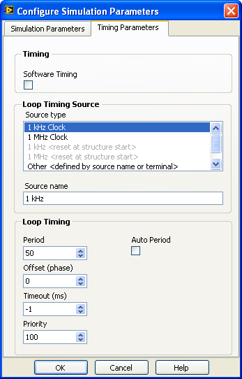
The Timing Parameters tab in the Configure Simulation Parameters dialog window
Comments to the Timing Parameters tab:
- The Period is the same as for the programmatic parameter settings describe above.
- The Software Timing is the same as for the programmatic settings described above. By default Software Timing is selected.
- If Auto Period is selected LabVIEW automatically sets the period of the simulation equal to the simulation time step. By default Auto Period is not selected.
| Run the VI. Hopefully it works. |
5 Various topics
(There are no blue activity boxes in Chapter.)
5.1 Representing state space models using Formula node and integrators
A state-space model is a set of first order differential equations constituting the model of the system. State-space models is a standardized model form. It is common that mathematical models of dynamic systems are written as state-space models. To be a little more specific, here is a general second order state-space model (the dots represents the arguments of the functions):
dx1/dt = f1(x1,x2,...)
dx2/dt = f2(x1,x2,...)
y = g(x1,x2,...)
where f1(•) and f2(•) are functions containing the right-hand part of the first order differential equations. The arguments may be state variables, input variables, and parameters. These functions may be linear or nonlinear. They are the time-derivatives of the states, x1 and x2, respectively. Sometimes one or more output variables are defined. Above, the output variable is y, and the output function is g(•).
To implement the block diagram of a state-space model, you may start by adding one Integrator block for each of the state variables on the block diagram. The output of the integrators are the state variables. The inputs to the integrators are the time derivatives, and the f1(•) and f2(•) functions in the representative model shown are these time derivatives. To implement the functions you have the following two options (which also may be combined):
- Constructing the functions, f1(•) and f2(•) above, using block functions as Sum, Gain, Multiplication etc., which are on the Simulation Palette of the Functions Palette. One example is the Block diagram of the model of the liquid tank shown here.
- Writing the textual functions of f1(•) and f2(•) in a Formula Node. The Formula node is on the Mathematics / Scripts & Formulas Palette (and on the Structures Palette). The Formula Node is explained here (in my Introduction to LabVIEW). With the Formula Node the functions are easier to modify (it is done by justing editing text in the Formula Node), and the Block Diagram may appear simpler. However, it may be difficult to implement nonlinear functions as hysteresis, backlash etc. (there are numerous such nonlinear blocks in the Nonlinear Palette on the Simulation Palette).
Here is a simple example of using the Formula node. Given the following state space model:
dx1/dt = x2
dx2/dt = -x1 + u
y = x1
(which is a state space model of an oscillator). u is the input variable, and y is the output variable. ssformulanode.vi shown below implements a simulator for this system. A Formula node is used to represent the right side of the differential equations. The integration of the time derivatives are performed by Integrator blocks from the Continuous palette.
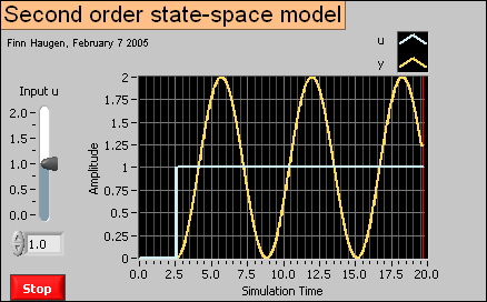
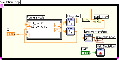
Front panel and block diagram of ssformulanode.vi.
Using Formula Node in stead of block functions to calculate the time derivatives may give a simpler block diagram. However, if the expressions for the time derivatives (i.e. the right-hand sides of the differential equations) contains nonlinear functions, it may be more difficult to implement these in the Formula Node than with function blocks.
5.2 Creating subsystems
You can create a subsystem of a part of a simulation diagram. The first step is to select or mark the part of interest, see the figure below, which shows the block diagram of tanksim.vi.
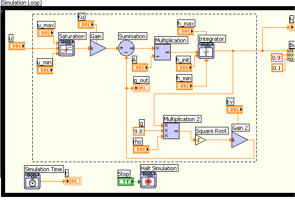
The first step in creating a subsystem in the simulation diagram is to select the part of interest
Then the subsystem is created using the menu . The resulting diagram is shown in the figure below.
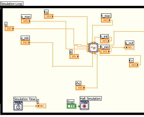
The resulting simulation diagram, including the subsystem
Note that you can change the size of the subsystem icon using the cursor.
If you want you can open the front panel of the subsystem by double-clicking the subsystem icon, see the figure below.
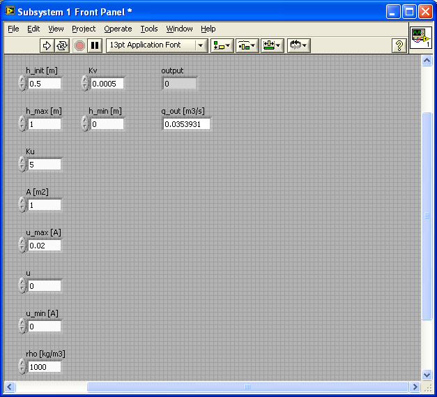
The front panel of the subsystem
You can open the block diagram of the subsystem via the menu, see the figure below.
The block diagram of the subsystem
5.3 Getting a linearized model of a subsystem
LabVIEW can create a linear state space model from a linear or nonlinear subsystem. (Creating subsystems is described in the previous section.) The procedure is to select or mark the subsystem of interest, and then create the linear model by using the following menu: . You are given the option of saving the linear model as a model (to be used by functions in the Control Design Toolkit) or as a VI containing the state space model in the form of a cluster of coefficient arrays. Perhaps the most flexible choice is VI.
5.4 Simulating control systems
Simulating control systems is done in the same way as simulating dynamic
systems. You can include virtually every control function in a model block
diagram inside the Simulation Loop. In Guidelines to
PID Control with
LabVIEW there is an example of a simulator of a PID control system.
5.5 Converting models between Simulation Module and Control Design Toolkit
You can convert models between the Simulation Module and the Control Design Toolkit using the conversion functions on the Model Conversion palette on the Control Design Tookit. The two conversion functions are shown in the figure below.
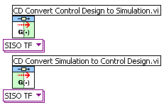
The conversion functions on the Control Design Toolkit / Model Conversion palette
5.6 Putting code into a While loop running in parallell with a Simulation loop
It is possible to put almost any LabVIEW code for e.g. analysis and design of into a simulation diagram inside a Simulation loop, but doing so may give an unnecessary large or complicated simulation code, and the simulation execution may be delayed. Therefore, you should not put more code inside the Simulation loop than is strictly necessary for representing the model to be simulated. Other parts of the total code, e.g. optimal control design functions (as the LQR function) or Kaman filter (state estimator) design functions (as the Kalman Gain function), may be put into one or more ordinary While loops running in parallel with the Simulation loop. These While loops may be programmed to run slower than the Simulation loop. Data can be exchanged between the loops using local variables (local variables are described in Introduction to LabVIEW).
Here is one example: kalmanfilter_tank.vi is a simulator of a Kalman Filter which estimates the outflow of a simulated liquid tank. (You can run this simulator if you have the LabVIEW Simulation Module installed.) The simulator is implemented with a Simulation Loop which contains a model of the tank and the expressions constituting the Kalman Filter algorithm. The Kalman gains are calculated using the Kalman Gain function of the Control Design Toolkit. This function is relatively computational demanding, and it is therefore put into a While loop which runs in parallell with the Simulation loop with a cycle time of 0.5 sec. The Kalman gains are made available inside the Simulation loop using local variables.
The simulation time step is 0.1 sec, and the Period (which is the actual, real time that LabVIEW used to proceed one simulation time step) is 0.025 sec. (Having the Period smaller than the simulation time step makes the simulator run faster than real time. This is favourable here since the process itself is a slow system, and we do not have time to sit waiting for responses to come.) If we had put the Kalman Gain function inside the Simulation loop, the specified Period of 0.025 sec could not have been obtained because it takes about 0.3 sec (this is however computer-dependent) to execute Kalman Gain function.
Below are the front panel and the block diagram of kalmanfilter_tank.vi. Click on the figures to see them in full sizes. Note how local variables are used to exchange values across the loops. Note also how the Stop button and its local variable is used to stop both loops. The Mechanical Action property of the Stop button must be set to Switch until Released. If it is set to one of the Latch... properties, it it will not be possible to create local variable for it.)
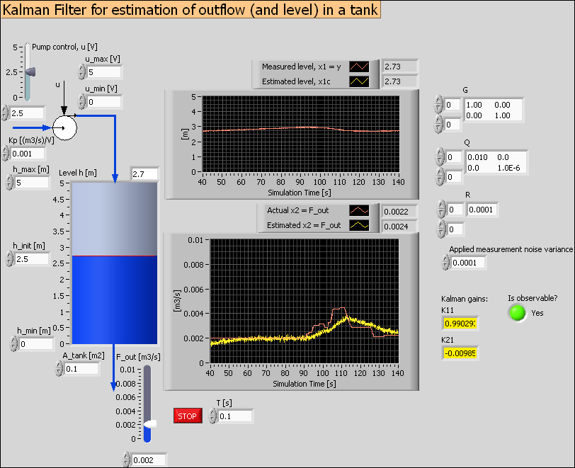
Front panel of kalmanfilter_tank.vi
Block diagram of kalmanfilter_tank.vi
5.7 Translating SIMULINK models into LabVIEW Simulation Module models
You can translate SIMULINK (MathWorks) models into LabVIEW simulation models using the menu Tools / Simulation Tools / SIMULINK Translator in LabVIEW.